국비지원교육/교육일지

1주차: 통계학 기초이론 및 선형대수, 보스턴 데이터분석

민서타 2023. 7. 21. 12:04

두줄요약:

기존 산업공학을 전공해서 대부분의 개념은 이해하고 있지만,

자주 쓰이는 이론 위주로 되새기며 복습하는 시간을 가지게 되었다.

확률: 0과 1사이의 사건이 일어날 확률

베르누이분포: 성공이면 1 실패하면 0의 값을 갖는 확률변수의 분포

이항분포: 베르누이 시행을 n번 독립 시행한 분포

가설과 검증:

제 1종 오류: 귀무가설이 옳은데도 불구하고 이를 기각

제 2종 오류: 귀무가설이 옳지 않은데도 이를 채택

혼동행렬(Confusion Matrix)

예측
실제		Positive	Negative
	Poistive	TP	FN	민감도 TP/(TP+FN)
	Negative	FP	TN	특이도 TN/(TN+FP)
		정밀도 TP/(TP+FP)	Negative Pvalue TN/(TN+FN)	정확도 TP+TN/ (TP+TN+FP+FN)

2. 선형대수학(1):

행렬과 선형 방정식

1) 가우스 소거 방식:

첨가 행렬: 선형 시스템의 상수 부분만 모아서 행렬 형태로 나타낸 것 / 연립방정식(선형시스템) 가정

가우스 행렬: 각 행의 첫 원소는 1이고, 1 아래에 위치하는 원소는 모두 0인 행렬

가우스 소거법 풀이(기본 행 연산):

-한 행에 0이 아닌 상수를 모두 곱하기 or 나누기

-두 행을 교환한다

-한 행의 배수를 다른 행에 더한다

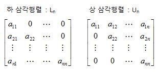
1. 삼각 행렬

  ㅇ 주 대각선 위 또는 아래 성분들 모두가 0 인 정방행렬


2. 삼각 행렬의 종류

  ㅇ 하 삼각행렬 (Lower Triangular Matrix) : Ln
     - 주대각선 위의 모든 성분이 0 인 정방행렬

  ㅇ 상 삼각행렬 (Upper Triangular Matrix) : Un
     - 주대각선 아래의 모든 성분이 0 인 정방행렬

In [1]:

import numpy as np
import pandas as pd
import seaborn as sns
import matplotlib.pyplot as plt
import statsmodels.api as sm

from math import sqrt
from sklearn import preprocessing
from sklearn import datasets
from sklearn.linear_model import LinearRegression
from sklearn.model_selection import train_test_split
from sklearn.metrics import mean_squared_error
from statsmodels.stats.outliers_influence import variance_inflation_factor
from IPython.core.display import display, HTML #주피터노트북 티스토리 업로드방법
display(HTML("")) #프린트 미리보기 선택,

C:\Users\user\AppData\Local\Temp\ipykernel_25020\1336359969.py:14: DeprecationWarning: Importing display from IPython.core.display is deprecated since IPython 7.14, please import from IPython display
  from IPython.core.display import display, HTML

In [2]:

dataset = pd.read_csv('boston1.csv')

In [3]:

dataset.describe()

Out[3]:

	CRIM	ZN	INDUS	CHAS	NOX	RM	AGE	DIS	RAD	TAX	PTRATIO	B	LSTAT	MEDV	CAT. MEDV
count	506.000000	506.000000	506.000000	506.000000	506.000000	506.000000	506.000000	506.000000	506.000000	506.000000	506.000000	506.000000	506.000000	506.000000	506.000000
mean	3.613524	11.363636	11.136779	0.069170	0.554695	6.284634	68.574901	3.795043	9.549407	408.237154	18.455534	356.674032	12.653063	22.532806	0.166008
std	8.601545	23.322453	6.860353	0.253994	0.115878	0.702617	28.148861	2.105710	8.707259	168.537116	2.164946	91.294864	7.141062	9.197104	0.372456
min	0.006320	0.000000	0.460000	0.000000	0.385000	3.561000	2.900000	1.129600	1.000000	187.000000	12.600000	0.320000	1.730000	5.000000	0.000000
25%	0.082045	0.000000	5.190000	0.000000	0.449000	5.885500	45.025000	2.100175	4.000000	279.000000	17.400000	375.377500	6.950000	17.025000	0.000000
50%	0.256510	0.000000	9.690000	0.000000	0.538000	6.208500	77.500000	3.207450	5.000000	330.000000	19.050000	391.440000	11.360000	21.200000	0.000000
75%	3.677083	12.500000	18.100000	0.000000	0.624000	6.623500	94.075000	5.188425	24.000000	666.000000	20.200000	396.225000	16.955000	25.000000	0.000000
max	88.976200	100.000000	27.740000	1.000000	0.871000	8.780000	100.000000	12.126500	24.000000	711.000000	22.000000	396.900000	37.970000	50.000000	1.000000

In [4]:

dataset.shape

Out[4]:

(506, 15)

In [5]:

dt = dataset.copy()

In [6]:

dt.isnull().sum() #결측치 없음

Out[6]:

CRIM         0
ZN           0
INDUS        0
CHAS         0
NOX          0
RM           0
AGE          0
DIS          0
RAD          0
TAX          0
PTRATIO      0
B            0
LSTAT        0
MEDV         0
CAT. MEDV    0
dtype: int64

In [7]:

dt.head()

Out[7]:

	CRIM	ZN	INDUS	NOX	RM	AGE	DIS	RAD	TAX	PTRATIO	B	LSTAT	MEDV	CAT. MEDV
0	0.00632	18.0	2.31	0.538	6.575	65.2	4.0900	1	296	15.3	396.90	4.98	24.0	0
1	0.02731	0.0	7.07	0.469	6.421	78.9	4.9671	2	242	17.8	396.90	9.14	21.6	0
2	0.02729	0.0	7.07	0.469	7.185	61.1	4.9671	2	242	17.8	392.83	4.03	34.7	1
3	0.03237	0.0	2.18	0.458	6.998	45.8	6.0622	3	222	18.7	394.63	2.94	33.4	1
4	0.06905	0.0	2.18	0.458	7.147	54.2	6.0622	3	222	18.7	396.90	5.33	36.2	1

In [8]:

dt.columns.to_frame()

Out[8]:

	0
CRIM	CRIM
ZN	ZN
INDUS	INDUS
CHAS	CHAS
NOX	NOX
RM	RM
AGE	AGE
DIS	DIS
RAD	RAD
TAX	TAX
PTRATIO	PTRATIO
B	B
LSTAT	LSTAT
MEDV	MEDV
CAT. MEDV	CAT. MEDV

In [9]:

dt_x =dt.loc[:, ('CRIM', 'ZN', 'INDUS', 'CHAS', 'NOX', 'RM', 'AGE', 'DIS', 'RAD', 'TAX',
       'PTRATIO', 'B', 'LSTAT')]
dt_y = dt.loc[:, ('MEDV')].to_frame()
df = pd.concat([dt_x, dt_y], axis=1)

Min-Max Scaler 적용(범주형 변수 제외)¶

In [10]:

df.columns

Out[10]:

Index(['CRIM', 'ZN', 'INDUS', 'CHAS', 'NOX', 'RM', 'AGE', 'DIS', 'RAD', 'TAX',
       'PTRATIO', 'B', 'LSTAT', 'MEDV'],
      dtype='object')

In [11]:

min_max_scaler = preprocessing.MinMaxScaler()
scale_col = ['CRIM', 'ZN', 'INDUS', 'NOX', 'RM', 'AGE', 'DIS', 'RAD', 'TAX',
       'PTRATIO', 'B', 'LSTAT']
df[scale_col] = min_max_scaler.fit_transform(dt_x[scale_col])

In [12]:

dt_x.describe()

Out[12]:

	CRIM	ZN	INDUS	CHAS	NOX	RM	AGE	DIS	RAD	TAX	PTRATIO	B	LSTAT
count	506.000000	506.000000	506.000000	506.000000	506.000000	506.000000	506.000000	506.000000	506.000000	506.000000	506.000000	506.000000	506.000000
mean	3.613524	11.363636	11.136779	0.069170	0.554695	6.284634	68.574901	3.795043	9.549407	408.237154	18.455534	356.674032	12.653063
std	8.601545	23.322453	6.860353	0.253994	0.115878	0.702617	28.148861	2.105710	8.707259	168.537116	2.164946	91.294864	7.141062
min	0.006320	0.000000	0.460000	0.000000	0.385000	3.561000	2.900000	1.129600	1.000000	187.000000	12.600000	0.320000	1.730000
25%	0.082045	0.000000	5.190000	0.000000	0.449000	5.885500	45.025000	2.100175	4.000000	279.000000	17.400000	375.377500	6.950000
50%	0.256510	0.000000	9.690000	0.000000	0.538000	6.208500	77.500000	3.207450	5.000000	330.000000	19.050000	391.440000	11.360000
75%	3.677083	12.500000	18.100000	0.000000	0.624000	6.623500	94.075000	5.188425	24.000000	666.000000	20.200000	396.225000	16.955000
max	88.976200	100.000000	27.740000	1.000000	0.871000	8.780000	100.000000	12.126500	24.000000	711.000000	22.000000	396.900000	37.970000

In [13]:

df.describe()

Out[13]:

	CRIM	ZN	INDUS	CHAS	NOX	RM	AGE	DIS	RAD	TAX	PTRATIO	B	LSTAT	MEDV
count	506.000000	506.000000	506.000000	506.000000	506.000000	506.000000	506.000000	506.000000	506.000000	506.000000	506.000000	506.000000	506.000000	506.000000
mean	0.040544	0.113636	0.391378	0.069170	0.349167	0.521869	0.676364	0.242381	0.371713	0.422208	0.622929	0.898568	0.301409	22.532806
std	0.096679	0.233225	0.251479	0.253994	0.238431	0.134627	0.289896	0.191482	0.378576	0.321636	0.230313	0.230205	0.197049	9.197104
min	0.000000	0.000000	0.000000	0.000000	0.000000	0.000000	0.000000	0.000000	0.000000	0.000000	0.000000	0.000000	0.000000	5.000000
25%	0.000851	0.000000	0.173387	0.000000	0.131687	0.445392	0.433831	0.088259	0.130435	0.175573	0.510638	0.945730	0.144040	17.025000
50%	0.002812	0.000000	0.338343	0.000000	0.314815	0.507281	0.768280	0.188949	0.173913	0.272901	0.686170	0.986232	0.265728	21.200000
75%	0.041258	0.125000	0.646628	0.000000	0.491770	0.586798	0.938980	0.369088	1.000000	0.914122	0.808511	0.998298	0.420116	25.000000
max	1.000000	1.000000	1.000000	1.000000	1.000000	1.000000	1.000000	1.000000	1.000000	1.000000	1.000000	1.000000	1.000000	50.000000

In [14]:

X_train, X_test, y_train, y_test = train_test_split(dt_x, dt_y, test_size = 0.3)
print(len(X_train), len(X_test), len(y_train), len(y_test))

354 152 354 152

In [15]:

X_train.head()

Out[15]:

	CRIM	INDUS	NOX	RM	AGE	DIS	RAD	TAX	PTRATIO	B	LSTAT
400	25.04610	18.10	0.693	5.987	100.0	1.5888	24	666	20.2	396.90	26.77
342	0.02498	1.89	0.518	6.540	59.7	6.2669	1	422	15.9	389.96	8.65
232	0.57529	6.20	0.507	8.337	73.3	3.8384	8	307	17.4	385.91	2.47
127	0.25915	21.89	0.624	5.693	96.0	1.7883	4	437	21.2	392.11	17.19
476	4.87141	18.10	0.614	6.484	93.6	2.3053	24	666	20.2	396.21	18.68

In [16]:

y_train

Out[16]:

	MEDV
400	5.6
342	16.5
232	41.7
127	16.2
476	16.7
...	...
311	22.1
131	19.6
289	24.8
227	31.6
407	27.9

354 rows × 1 columns

In [17]:

model_reg = sm.OLS(y_train, X_train).fit() #y값 먼저 대입필요
print(model_reg.summary())

                                 OLS Regression Results                                
=======================================================================================
Dep. Variable:                   MEDV   R-squared (uncentered):                   0.962
Model:                            OLS   Adj. R-squared (uncentered):              0.961
Method:                 Least Squares   F-statistic:                              667.1
Date:                Fri, 21 Jul 2023   Prob (F-statistic):                   1.97e-233
Time:                        16:11:48   Log-Likelihood:                         -1048.2
No. Observations:                 354   AIC:                                      2122.
Df Residuals:                     341   BIC:                                      2173.
Df Model:                          13                                                  
Covariance Type:            nonrobust                                                  
==============================================================================
                 coef    std err          t      P>|t|      [0.025      0.975]
------------------------------------------------------------------------------
CRIM          -0.1001      0.035     -2.874      0.004      -0.169      -0.032
ZN             0.0405      0.017      2.434      0.015       0.008       0.073
INDUS          0.0257      0.076      0.339      0.734      -0.123       0.174
CHAS           2.9881      1.091      2.739      0.006       0.842       5.134
NOX           -2.1319      3.927     -0.543      0.588      -9.856       5.592
RM             6.2498      0.359     17.389      0.000       5.543       6.957
AGE           -0.0101      0.016     -0.630      0.529      -0.042       0.021
DIS           -0.8189      0.224     -3.650      0.000      -1.260      -0.378
RAD            0.1560      0.073      2.122      0.035       0.011       0.301
TAX           -0.0081      0.004     -1.835      0.067      -0.017       0.001
PTRATIO       -0.4639      0.123     -3.760      0.000      -0.707      -0.221
B              0.0091      0.003      2.813      0.005       0.003       0.015
LSTAT         -0.4186      0.057     -7.281      0.000      -0.532      -0.305
==============================================================================
Omnibus:                      131.270   Durbin-Watson:                   2.041
Prob(Omnibus):                  0.000   Jarque-Bera (JB):              549.927
Skew:                           1.566   Prob(JB):                    3.85e-120
Kurtosis:                       8.241   Cond. No.                     8.68e+03
==============================================================================

Notes:
[1] R² is computed without centering (uncentered) since the model does not contain a constant.
[2] Standard Errors assume that the covariance matrix of the errors is correctly specified.
[3] The condition number is large, 8.68e+03. This might indicate that there are
strong multicollinearity or other numerical problems.

In [18]:

y_pred = np.array(model_reg.predict(X_test))
y_pred.shape[0]

Out[18]:

In [19]:

y_pred = y_pred.reshape(y_pred.shape[0], 1)
y_test = np.array(y_test)
print(mean_squared_error(y_test, y_pred))

30.788484245031093

In [20]:

X_test.corr()

Out[20]:

	CRIM	ZN	INDUS	CHAS	NOX	RM	AGE	DIS	RAD	TAX	PTRATIO	B	LSTAT
CRIM	1.000000	-0.244676	0.518364	-0.043134	0.530430	-0.290115	0.485451	-0.449761	0.754123	0.728520	0.360045	-0.323776	0.615932
ZN	-0.244676	1.000000	-0.549438	0.020785	-0.494083	0.347975	-0.540511	0.674015	-0.319197	-0.303907	-0.455233	0.153693	-0.435898
INDUS	0.518364	-0.549438	1.000000	0.144864	0.776237	-0.424840	0.642520	-0.692970	0.612403	0.673771	0.414862	-0.338386	0.667472
CHAS	-0.043134	0.020785	0.144864	1.000000	0.232119	0.068162	0.066910	-0.116841	-0.035787	-0.002682	-0.207308	-0.018106	-0.063804
NOX	0.530430	-0.494083	0.776237	0.232119	1.000000	-0.320289	0.737130	-0.753488	0.595612	0.652228	0.184858	-0.387749	0.655328
RM	-0.290115	0.347975	-0.424840	0.068162	-0.320289	1.000000	-0.266352	0.214858	-0.193380	-0.276566	-0.341932	-0.041500	-0.632443
AGE	0.485451	-0.540511	0.642520	0.066910	0.737130	-0.266352	1.000000	-0.749512	0.503010	0.514308	0.308943	-0.264063	0.649008
DIS	-0.449761	0.674015	-0.692970	-0.116841	-0.753488	0.214858	-0.749512	1.000000	-0.478152	-0.492158	-0.267999	0.244703	-0.554035
RAD	0.754123	-0.319197	0.612403	-0.035787	0.595612	-0.193380	0.503010	-0.478152	1.000000	0.945726	0.495882	-0.420105	0.482526
TAX	0.728520	-0.303907	0.673771	-0.002682	0.652228	-0.276566	0.514308	-0.492158	0.945726	1.000000	0.475039	-0.420468	0.542458
PTRATIO	0.360045	-0.455233	0.414862	-0.207308	0.184858	-0.341932	0.308943	-0.267999	0.495882	0.475039	1.000000	-0.163091	0.358083
B	-0.323776	0.153693	-0.338386	-0.018106	-0.387749	-0.041500	-0.264063	0.244703	-0.420105	-0.420468	-0.163091	1.000000	-0.298589
LSTAT	0.615932	-0.435898	0.667472	-0.063804	0.655328	-0.632443	0.649008	-0.554035	0.482526	0.542458	0.358083	-0.298589	1.000000

In [21]:

plt.figure(figsize=(10, 8))
sns.heatmap(X_train.corr(), annot = True, cmap = 'RdYlBu')
plt.show()

다중공선성 vif 확인¶

In [22]:

tmp_train_X1 = X_train.drop('TAX', axis=1)
tmp_train_X1
vif = pd.DataFrame()
vif["VIF Factor"] = [variance_inflation_factor(tmp_train_X1.values, i) for i in range(tmp_train_X1.shape[1])]
vif["features"] = tmp_train_X1.columns
vif

Out[22]:

	VIF Factor	features
0	2.022017	CRIM
1	2.651376	ZN
2	11.351344	INDUS
3	1.132375	CHAS
4	75.552423	NOX
5	80.220503	RM
6	22.029156	AGE
7	15.203582	DIS
8	5.561729	RAD
9	79.602360	PTRATIO
10	21.747249	B
11	10.706293	LSTAT

In [23]:

train_x_tmp = X_train[vif['features']]
model_reg2 = sm.OLS(y_train, train_x_tmp).fit()
print(model_reg2.summary())

                                 OLS Regression Results                                
=======================================================================================
Dep. Variable:                   MEDV   R-squared (uncentered):                   0.962
Model:                            OLS   Adj. R-squared (uncentered):              0.960
Method:                 Least Squares   F-statistic:                              717.5
Date:                Fri, 21 Jul 2023   Prob (F-statistic):                   3.83e-234
Time:                        16:11:49   Log-Likelihood:                         -1049.9
No. Observations:                 354   AIC:                                      2124.
Df Residuals:                     342   BIC:                                      2170.
Df Model:                          12                                                  
Covariance Type:            nonrobust                                                  
==============================================================================
                 coef    std err          t      P>|t|      [0.025      0.975]
------------------------------------------------------------------------------
CRIM          -0.0998      0.035     -2.855      0.005      -0.169      -0.031
ZN             0.0336      0.016      2.066      0.040       0.002       0.066
INDUS         -0.0442      0.066     -0.675      0.500      -0.173       0.085
CHAS           3.2677      1.084      3.014      0.003       1.135       5.400
NOX           -2.8949      3.918     -0.739      0.461     -10.602       4.812
RM             6.2309      0.361     17.284      0.000       5.522       6.940
AGE           -0.0112      0.016     -0.695      0.487      -0.043       0.020
DIS           -0.8417      0.225     -3.744      0.000      -1.284      -0.400
RAD            0.0519      0.047      1.107      0.269      -0.040       0.144
PTRATIO       -0.5043      0.122     -4.139      0.000      -0.744      -0.265
B              0.0090      0.003      2.800      0.005       0.003       0.015
LSTAT         -0.4215      0.058     -7.309      0.000      -0.535      -0.308
==============================================================================
Omnibus:                      127.587   Durbin-Watson:                   2.050
Prob(Omnibus):                  0.000   Jarque-Bera (JB):              512.677
Skew:                           1.533   Prob(JB):                    4.72e-112
Kurtosis:                       8.035   Cond. No.                     5.77e+03
==============================================================================

Notes:
[1] R² is computed without centering (uncentered) since the model does not contain a constant.
[2] Standard Errors assume that the covariance matrix of the errors is correctly specified.
[3] The condition number is large, 5.77e+03. This might indicate that there are
strong multicollinearity or other numerical problems.

In [24]:

train_x_tmp

Out[24]:

	CRIM	ZN	INDUS	CHAS	NOX	RM	AGE	DIS	RAD	PTRATIO	B	LSTAT
400	25.04610	0.0	18.10	0	0.693	5.987	100.0	1.5888	24	20.2	396.90	26.77
342	0.02498	0.0	1.89	0	0.518	6.540	59.7	6.2669	1	15.9	389.96	8.65
232	0.57529	0.0	6.20	0	0.507	8.337	73.3	3.8384	8	17.4	385.91	2.47
127	0.25915	0.0	21.89	0	0.624	5.693	96.0	1.7883	4	21.2	392.11	17.19
476	4.87141	0.0	18.10	0	0.614	6.484	93.6	2.3053	24	20.2	396.21	18.68
...	...	...	...	...	...	...	...	...	...	...	...	...
311	0.79041	0.0	9.90	0	0.544	6.122	52.8	2.6403	4	18.4	396.90	5.98
131	1.19294	0.0	21.89	0	0.624	6.326	97.7	2.2710	4	21.2	396.90	12.26
289	0.04297	52.5	5.32	0	0.405	6.565	22.9	7.3172	6	16.6	371.72	9.51
227	0.41238	0.0	6.20	0	0.504	7.163	79.9	3.2157	8	17.4	372.08	6.36
407	11.95110	0.0	18.10	0	0.659	5.608	100.0	1.2852	24	20.2	332.09	12.13

354 rows × 12 columns

In [25]:

tmp_train_X2 = tmp_train_X1.drop(['AGE','NOX','INDUS','RAD'], axis=1)
vif = pd.DataFrame()
vif["VIF Factor"] = [variance_inflation_factor(tmp_train_X2.values, i) for i in range(tmp_train_X2.shape[1])]
vif["features"] = tmp_train_X2.columns
vif

Out[25]:

	VIF Factor	features
0	1.684411	CRIM
1	2.561421	ZN
2	1.111489	CHAS
3	49.152663	RM
4	9.366985	DIS
5	64.289267	PTRATIO
6	20.035466	B
7	7.269728	LSTAT

In [26]:

train_x_tmp2 = X_train[vif['features'].tolist()]
model_reg2 = sm.OLS(y_train, train_x_tmp2).fit()
print(model_reg2.summary())

                                 OLS Regression Results                                
=======================================================================================
Dep. Variable:                   MEDV   R-squared (uncentered):                   0.961
Model:                            OLS   Adj. R-squared (uncentered):              0.961
Method:                 Least Squares   F-statistic:                              1077.
Date:                Fri, 21 Jul 2023   Prob (F-statistic):                   2.40e-239
Time:                        16:11:49   Log-Likelihood:                         -1051.7
No. Observations:                 354   AIC:                                      2119.
Df Residuals:                     346   BIC:                                      2150.
Df Model:                           8                                                  
Covariance Type:            nonrobust                                                  
==============================================================================
                 coef    std err          t      P>|t|      [0.025      0.975]
------------------------------------------------------------------------------
CRIM          -0.0851      0.032     -2.668      0.008      -0.148      -0.022
ZN             0.0375      0.016      2.347      0.019       0.006       0.069
CHAS           3.3270      1.073      3.100      0.002       1.216       5.438
RM             5.9494      0.282     21.097      0.000       5.395       6.504
DIS           -0.6737      0.176     -3.821      0.000      -1.020      -0.327
PTRATIO       -0.5219      0.109     -4.770      0.000      -0.737      -0.307
B              0.0079      0.003      2.550      0.011       0.002       0.014
LSTAT         -0.4700      0.047     -9.898      0.000      -0.563      -0.377
==============================================================================
Omnibus:                      126.928   Durbin-Watson:                   2.069
Prob(Omnibus):                  0.000   Jarque-Bera (JB):              488.203
Skew:                           1.543   Prob(JB):                    9.73e-107
Kurtosis:                       7.855   Cond. No.                     1.56e+03
==============================================================================

Notes:
[1] R² is computed without centering (uncentered) since the model does not contain a constant.
[2] Standard Errors assume that the covariance matrix of the errors is correctly specified.
[3] The condition number is large, 1.56e+03. This might indicate that there are
strong multicollinearity or other numerical problems.

In [27]:

X_train, X_test, y_train, y_test = train_test_split(dt_x, dt_y, test_size = 0.3)

In [28]:

test_X = X_test[train_x_tmp2.columns.tolist()]
pred_y = np.array(model_reg2.predict(test_X)).reshape(test_X.shape[0], 1)
test_y = np.array(y_test)
print(mean_squared_error(test_y, pred_y))

29.170495164279384

In [29]:

plt.plot(pred_y, label = 'pred')
plt.plot(test_y, label = 'true')
plt.legend()
plt.show()

In [30]:

pred_y

Out[30]:

array([[16.94550911],
       [17.06318997],
       [20.54065983],
       [21.49509505],
       [17.842118  ],
       [12.58932649],
       [31.31908622],
       [17.14226678],
       [27.22801086],
       [12.233781  ],
       [31.94042244],
       [21.17474098],
       [16.32947821],
       [21.19142718],
       [19.69822565],
       [20.20106887],
       [19.62960322],
       [19.95144895],
       [21.59235344],
       [25.44674209],
       [18.42501619],
       [21.8482483 ],
       [23.04676536],
       [18.75243435],
       [45.15338169],
       [18.27825643],
       [24.45879603],
       [21.57348341],
       [19.74667716],
       [40.46712952],
       [26.75884084],
       [14.02397676],
       [16.64543724],
       [ 9.371997  ],
       [19.81640339],
       [17.51593477],
       [ 7.12945118],
       [23.0862328 ],
       [21.73210393],
       [19.21173085],
       [21.83106448],
       [24.40072858],
       [22.98499848],
       [20.55485757],
       [22.77185682],
       [-1.58167649],
       [25.66895708],
       [17.05482392],
       [38.02223795],
       [21.13824977],
       [22.65369217],
       [25.44076153],
       [16.39568516],
       [31.11180702],
       [20.48406463],
       [30.27113734],
       [20.54221571],
       [17.9006872 ],
       [21.48640082],
       [19.62053209],
       [23.74390288],
       [21.87764934],
       [34.01615951],
       [35.62375702],
       [12.17641457],
       [23.27824859],
       [28.29387189],
       [36.19784489],
       [13.63754619],
       [26.77559107],
       [20.32009368],
       [19.27941465],
       [20.86134972],
       [ 8.84693351],
       [21.97829917],
       [28.82398194],
       [24.12401008],
       [19.73771985],
       [31.83150742],
       [18.94242343],
       [38.12771144],
       [20.05306732],
       [21.38847832],
       [25.08723355],
       [21.91955087],
       [20.42587881],
       [11.52379919],
       [13.29226738],
       [17.59421761],
       [33.59897801],
       [15.15158945],
       [32.97827089],
       [13.3349062 ],
       [35.43021454],
       [17.88616598],
       [23.10416616],
       [16.79790539],
       [19.06132253],
       [20.12735175],
       [18.89815349],
       [32.05918937],
       [23.2078107 ],
       [22.59919457],
       [15.0472258 ],
       [25.13964369],
       [17.37588045],
       [18.07303403],
       [16.66295959],
       [25.75617075],
       [16.46914616],
       [19.14471539],
       [34.74453313],
       [32.29757376],
       [21.79677393],
       [27.01993766],
       [30.01671501],
       [25.98306658],
       [18.38125739],
       [21.46336421],
       [21.43943523],
       [25.40031236],
       [18.93182955],
       [18.64059264],
       [22.27972866],
       [24.84748359],
       [26.24849258],
       [26.82331438],
       [ 6.39062658],
       [20.23056685],
       [26.26349633],
       [26.96599772],
       [20.90609139],
       [36.1485794 ],
       [17.70159442],
       [39.82916123],
       [14.53002613],
       [26.95571339],
       [31.91391993],
       [26.48773934],
       [12.42796913],
       [20.91309803],
       [25.89308065],
       [39.12853701],
       [23.0499243 ],
       [27.03465854],
       [31.32979802],
       [22.54633642],
       [21.93128173],
       [27.90272931],
       [17.97826182],
       [23.38359188],
       [21.55268912]])

'국비지원교육 > 교육일지' 카테고리의 다른 글

6주차 교육일지: 코딩 테스트 주요 개념, Git 설정, 마크다운 (0)	2023.09.11
5주차 교육일지: Pandas feature engineering (0)	2023.08.21
4주차 교육일지: SQL / Numpy, Pandas (0)	2023.08.12
3주차 교육일지: 파이썬 기초, 선형대수, 웹크롤링 (0)	2023.07.31
2주차 교육일지: 파이썬 기초, 선형대수, 웹 크롤링 (0)	2023.07.24

현재글1주차: 통계학 기초이론 및 선형대수, 보스턴 데이터분석

패스트캠퍼스, DA, 딥러닝, 국비지원, AI, 민서타, 오블완, LLM, 민스타, 머신러닝, 태블로, 데이터분석, 추천시스템, It, nlp, 티스토리챌린지, 부트캠프, sql, 인공지능, DS,

Today :
Yesterday :

민서타의 데이터 분석 연구일지

1주차: 통계학 기초이론 및 선형대수, 보스턴 데이터분석

Min-Max Scaler 적용(범주형 변수 제외)¶

다중공선성 vif 확인¶

'국비지원교육 > 교육일지' 카테고리의 다른 글

'국비지원교육/교육일지'의 다른글

티스토리툴바

« 2025/05 »
일	월	화	수	목	금	토
				1	2	3
4	5	6	7	8	9	10
11	12	13	14	15	16	17
18	19	20	21	22	23	24
25	26	27	28	29	30	31

1주차: 통계학 기초이론 및 선형대수, 보스턴 데이터분석

Min-Max Scaler 적용(범주형 변수 제외)¶

다중공선성 vif 확인¶

'국비지원교육 > 교육일지' 카테고리의 다른 글

'국비지원교육/교육일지'의 다른글

관련글

티스토리툴바